dynagraph Templates
Download from http://www.math.umbc.edu/~rouben/dynagraph/download.
#Start dynagraph :
donsauer$ /sw/bin/dynagraph
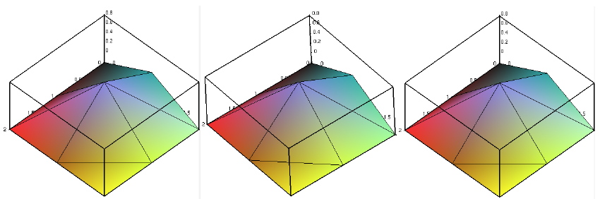
#Plot A File :
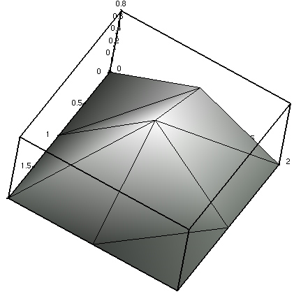
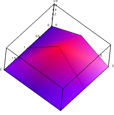
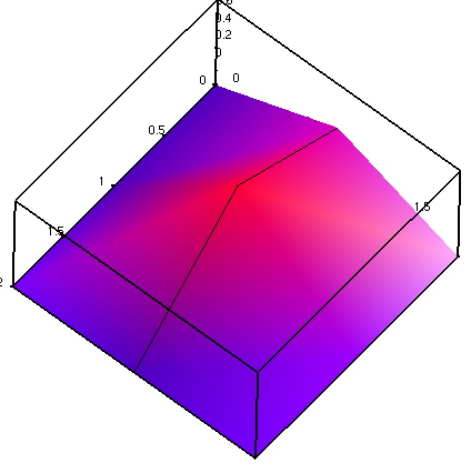
> dataplot(g432);
# ===========File g432===========================
# A surface defined on 3x3 grid. Plot with
# dataplot(filename);
# Also try dataplot(g432, gridstyle=triangular, style=patch);
# needs LF
# data as x0 y0 z0 x1 y1 z1...
SURF 3 3
0 0 0 0 1 0 0 2 0
1 0 0 1 1 1 1 2 0
2 0 0 2 1 0 2 2 0
# ==============================================
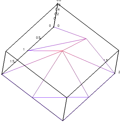
#Mouse Can Rotate the Graph :
dataplot(g432 , orientation=[45,95]);
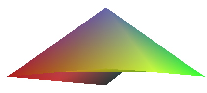
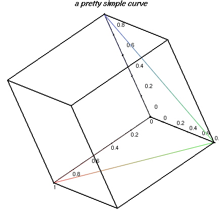
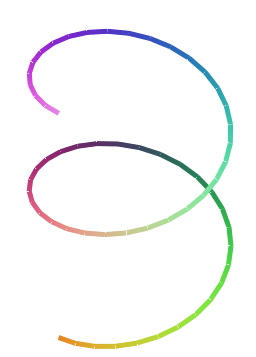
dataplot(g431,tuberadius=1/5);
# A simple closed curve: paste the following data
# into a file and plot with dataplot(g431);
TITLE "a pretty simple curve"
TUBE 5
0 0 0
1 0 0
0 1 0
0 0 1
0 0 0
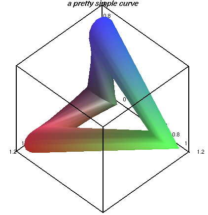
dataplot(g430);
# A simple closed curve: paste the following data
# into a file and plot with dataplot(g430);
TITLE "a pretty simple curve"
CURVE 5
0 0 0
1 0 0
0 1 0
0 0 1
0 0 0
sin cos tan # trigonometric functions
atan asin acos # inverse trigonometric functions
arctan arcsin arccos # synonyms of the above
atan2 # atan2(y,x) is similar to atan(y/x)
arctan2 # synonym of the above
sinh cosh tanh # hyperbolic functions
atanh asinh acosh # inverse hyperbolic functions
arctanh arcsinh arccosh # synonyms of the above
ln # the natural logarithm
log10 # logarithm in base 10
exp # the exponential function
erf erfc # error function and complementary error function
sqrt # square root
int # the integer part of a real number
abs # absolute value
BesselJ BesselY # Bessel functions of the first and second kind
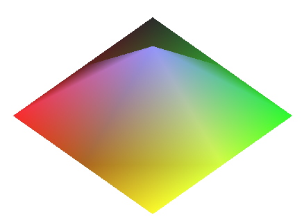
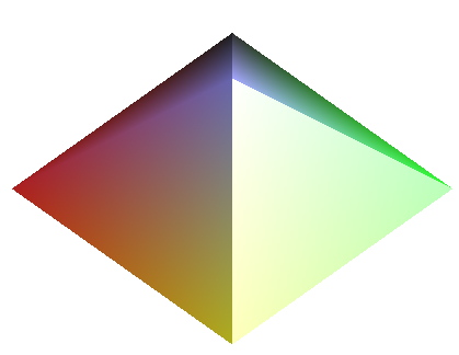
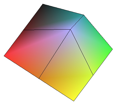
p1 := polygonplot([[-1,-1,1],[ 1,-1,1],[0,0,2]]):
p2 := polygonplot([[ 1,-1,1],[ 1, 1,1],[0,0,2]]):
p3 := polygonplot([[ 1, 1,1],[-1, 1,1],[0,0,2]]):
p4 := polygonplot([[-1, 1,1],[-1,-1,1],[0,0,2]]):
display([p1,p2,p3,p4]);
plot3d(x^2+y^2, x=-1..1, y=-1..1); # plot a curve:
plot3d(x^2-y^2, x=-1..1, y=-1..1); # plot another curve:
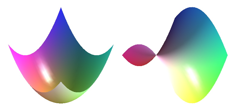
plot3d({x^2+y^2, x^2-y^2}, x=-1..1, y=-1..1); # plot two curves:
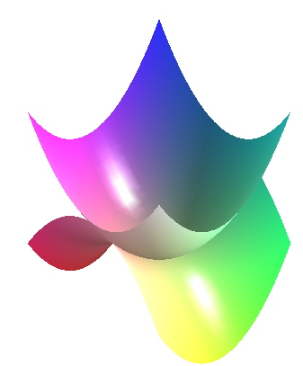
p1 := plot3d(x^2+y^2, x=-1..1, y=-1..1); # Assign p1:
p2 := plot3d(x^2-y^2, x=-1..1, y=-1..1); # Assign p2:
display({p1,p2}); # display both:
p3 := display({p1,p2}); # give the combined a name:
p1; # to display just p1:
r := sqrt(x^2+y^2); # assigns a statement :
plot3d(r, x=-1..1, y=-1..1); # plot a statement :
r; # show a statement :
(sqrt(x^2+y^2))
r := r; # remove a statement :
quit
dump; # displays symbol table. :
restart; # clears the symbol table. :
# Here is an helix :
p1 := spacecurve([cos(t),sin(t), t/4],
t=0..4*Pi,
thickness=5);
p1;
# Here is curve :
p2 := plot3d(x^2+y^2,
x=-1..1,
y=-1..1);
# Here is both :
display({p1,p2});
#quarterrd sphere:
plot3d([cos(t)*cos(s), cos(t)*sin(s), sin(t)],
t=0..2*Pi,
s=0..Pi/2);
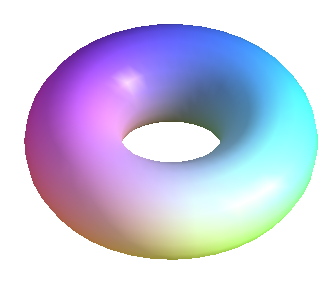
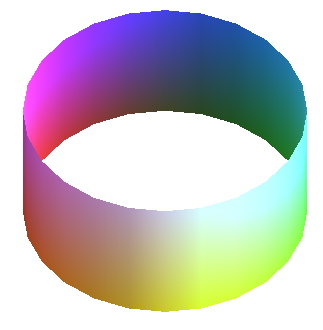
#donut:
plot3d([(2+cos(s))*cos(t), (2+cos(s))*sin(t), sin(s)],
t=0..2*Pi,
s=0..2*Pi,
grid=[40,20]);
#two curves:
plot3d({x^2+y^2, x^2-y^2},
x=-1..1,
y=-1..1);
#two curves:
plot3d({x^2+y^2, [x^2-y^2, x^2+y^2, x*y]},
x=-1..1,
y=-1..1);
#hemisphere:
plot3d( 1, s=0..2*Pi, t=0..Pi/2, coords=spherical);
#cylinder:
plot3d( 1, t=0..2*Pi, z=0..1, coords=cylindrical);
#paraboloid :
plot3d( r^2,
r=0..1,
t=0..2*Pi,
coords=z_cylindrical);
#Mobius strip:
plot3d( [ 1+v*cos(t/2), t, v*sin(t/2) ],
t=0..2*Pi,
v=-1/4..1/4,
grid=[100,3],
coords=z_cylindrical);
# vase:
plot3d([t+3*sin(t),
(4+3*cos(t))*cos(s),
(4+3*cos(t))*sin(s)],
s=0..3/2*Pi, t=0..4*Pi);
plot3d([t,
(3+sin(t))*cos(s),
(3+sin(t))*sin(s)],
s=0..2*Pi, t=0..4*Pi);
# helix:
spacecurve([cos(t),sin(t),t/4] ,t=0..4*Pi);
# helix2:
spacecurve( { [cos(t),sin(t),t/6], [sin(t),cos(t),t/6] },
t=0..4*Pi, thickness=4);
# helix:
p1 := spacecurve([cos(t),sin(t),t/4], t=0..4*Pi, thickness=5);
# parbola:
p2 := plot3d(x^2+y^2,x=-1..1,y=-1..1);
# both :
display([p1,p2]);
#donut:
tubeplot([cos(t), sin(t), 0], t=0..2*Pi, tuberadius=1/2);
tube twist
tubeplot({[cos(t), sin(t), t], [-cos(t), -sin(t), t]}, t=0..2*Pi);
#oolon statement doesnot plot :
p1 := polygonplot([[-1,-1,1],[1,-1,1],[0,0,2]]):
p2 := polygonplot([[1,-1,1],[1,1,1],[0,0,2]]):
p3 := polygonplot([[1,1,1],[-1,1,1],[0,0,2]]):
p4 := polygonplot([[-1,1,1],[-1,-1,1],[0,0,2]]):
#semicolon plots :
display([p1,p2,p3,p4]);
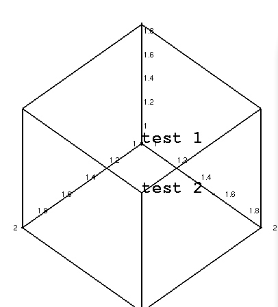
#textplot example:
p1 := textplot3d([1,1,1,"test 1"], color=red):
p2 := textplot3d([2,2,2,"test 2"], color=green):
display({p1, p2}, axes=boxed, font=[courier, bold, 24]);
p1 := plot3d(x^2+y^2,x=-1..1,y=-1..1);
p2 := plot3d(x^2-y^2,x=-1..1,y=-1..1);
display({p1, p2});
plot3d(x^2+y^2, x=-1..1, y=-1..1); # standard-issue paraboloid:
plot3d(x^2-y^2, x=-1..1, y=-1..1); # hyperboloid:
plot3d({x^2+y^2,x^2-y^2}, x=-1..1, y=-1..1); # two above together:
plot3d(r^2, r=0..1, t=0..2*Pi, coords=z_cylindrical); # paraboloid in cylindrical coordinates:
plot3d(z^2, t=0..2*Pi, z=0..1, coords=cylindrical); # inverse-paraboloid:
# torus:
p := plot3d([(2+cos(t))*cos(s),
(2+cos(t))*sin(s),sin(t)],
t=-Pi/2..Pi/2,
s=0..2*Pi,grid=[15,25]);
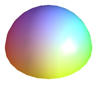
# sphere:
q := plot3d([1.5*sin(t)*cos(s),
1.5*sin(t)*sin(s),
1+1.5*cos(t)],
t=0..Pi/2,s=0..2*Pi) ;
# torus + sphere:
display([p,q]);
d1 := sqrt((x-1)^2+y^2); # Cassini oval1:
d2 := sqrt((x+1)^2+y^2); # Cassini oval2:
# Cassini surface:
plot3d(d1*d2,x=-2..2, y=-2..2,contours=60,
style=patchcontour,view=0..2);
# Clean Up:
d1 := d1; d2 := d2;
# atan2:
plot(atan2(y,x)/Pi, x=-1..1,y=-1..1, grid=[50,50],contours=30,style=patchcontour);
# Bessel zeroth order:
plot(5*BesselJ(0,r), r=0..8.6, t=0..1.5*Pi, coords=z_cylindrical);
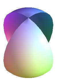
# Temple of Viviani:
R := 1:
a := 1.2;
sp := plot(R, s=0..2*Pi, t=0..Pi,
coords=spherical, grid=[60,60],color=brown):
cy := plot([R/2 + R/2*cos(t), R/2*sin(t), s],
t=0..2*Pi, s=-a*R..a*R,grid=[50,50], color=MediumPurple4):
tu := tubeplot([R/2 + R/2*cos(t), R/2*sin(t),
R*sin(t/2)], t=0..4*Pi,tuberadius=R/30, color=gold3, tubepoints=10):
display([sp,cy,tu],
title=`Temple of Viviani\n[ http://alem3d.obidos.org/en/struik/viviani/comm ]`);
R := R; a := a; sp := sp; cy := cy; tu := tu;
restart; # cleanup:
# dynagraph plots singularity at zero as a hole :
plot3d( x^2*y/(x^4+y^2),
x= -1..1,
y= -1..1,
style= patch);
^-- You goofed!
#zero no longer a mesh point:
plot3d(x^2*y/(x^4+y^2), x=-1..1, y=-1..1, style=patch, grid=[24,24]);
#anatomy:
plot3d(t,
t=-Pi..Pi,
s=0..Pi,
coords=spherical,
shading=zgrayscale,
title=anatomy);
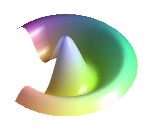
# torn sphere:
plot3d(t,
t=-Pi..Pi,
s=-Pi/2..Pi/2,
coords=spherical,
title=`a torn sphere`);
#shell 1:
plot3d([x*sin(x)*cos(y), x*cos(x)*cos(y), x*sin(y)],
x=0..2*Pi,
y=0..Pi,
title=`shell 1`);
#shell 2:
plot3d((1.3)^x * sin(y),
x=-1..2*Pi,
y=0..Pi,
coords=spherical,
title=`shell 2`);
# shell 3:
plot3d( theta,
theta= 0..3*Pi,
phi= Pi/12..Pi-Pi/12,
grid= [48,16],
coords= spherical,
title= `shell 3`);
# shell 4 :
plot3d([cos(u)*u*(1+cos(v)/2), sin(v)*u/2, sin(u)*u*(1+cos(v)/2)],
u=0..2*Pi,
v=0..2*Pi,
title=`shell 4`);
# a cone :
plot3d(z,
theta=0..2*Pi,
z=-5..5,
coords=cylindrical);
#real part of the complex square root function :
plot3d(r^(1/2)*cos(t/2),
r=0..1,
t=0..4*Pi,
grid=[10,50],
coords=z_cylindrical,
title=`Real part of the complex square root function`);
# real part of the complex cube root function:
plot3d(r^(1/3)*cos(t/3),
r=0..1,
t=0..6*Pi,
grid=[10,75],
coords=z_cylindrical,
title=`Real part of the complex cube root function`);
# Enneper's surface:
plot3d([u -u^3/3 + u*v^2,v -v^3/3 + v*u^2,u^2 - v^2],
u=-2..2,
v=-2..2,
title=`Enneper's surface`);
# Klein bottle:
x := (2*sin(u)*cos(v/2)-sin(2*u)*sin(v/2)+8)*cos(v):
y := (2*sin(u)*cos(v/2)-sin(2*u)*sin(v/2)+8)*sin(v):
z := 4*sin(u)*sin(v/2)+sin(2*u)*cos(v/2):
plot3d([x,y,z], u=0..2*Pi, v=0..2*Pi, grid=[20,40], title=`A Klein bottle`);
restart; # cleanup:
# Mobius strip:
w := 0.5;
n := 1;
r := 1 + v * cos(t*n/2);
z := v * sin(t*n/2);
plot3d([r,t,z],
t=0..2*Pi,
v=-w/2..w/2,
grid=[100,3],
coords=z_cylindrical);
restart; # cleanup:
# pointy sphere:
plot3d([cos(v)^3*cos(u)^3, sin(v)^3*cos(u)^3, sin(u)^3],
u=-Pi/2..Pi/2,
v=0..2*Pi,
title=`Sphere^3`);
restart; # cleanup:
#interlocking tori:
p := plot3d([cos(u)+0.5*cos(u)*cos(v),
sin(u)+0.5*sin(u)*cos(v), 0.5*sin(v)],
u=0..2*Pi,
v=0..2*Pi,
grid=[25,12]):
q := plot3d([1+cos(u)+.3*cos(u)*cos(v),
0.3*sin(v), sin(u)+0.3*sin(u)*cos(v)],
u=0..2*Pi,
v=0..2*Pi,
grid=[25,12]):
display([p,q]);
#interlocking circles:
spacecurve({[sin(t),0,cos(t)],[cos(t)+1,sin(t),0]},
t=-Pi..Pi,
thickness=5);
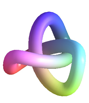
#knot:
u := -10*cos(t) - 2*cos(5*t) + 15*sin(2*t);
v := -15*cos(2*t) + 10*sin(t) - 2*sin(5*t);
w := 10*cos(3*t);
# plot as a spacecurve:
spacecurve([u,v,w],
t= 0..2*Pi);
# plot as a tube:
tubeplot([u,v,w],
t= 0..2*Pi,
tuberadius=4,
tubepoints=20,
numpoints=100);
restart; # cleanup:
#coil spring:
n := 4;
R := 5;
p0 := tubeplot([R*cos(t), R*sin(t), 0], t=0..2*Pi, numpoints=25);
p1 := tubeplot([R*cos(t), R*sin(t), t], t=0..2*n*Pi, numpoints=25*n);
p2 := tubeplot([R*cos(t), R*sin(t), 2*n*Pi], t=0..2*Pi, numpoints=25);
display([p0,p1,p2], title=`a coil spring`);
restart; # cleanup:
#trefoil around a torus:
a := 4; b := 2; c := 2; p := 2; q := 3;
knot := spacecurve([(a + b*cos(q*t))*cos(p*t),
(a + b*cos(q*t))*sin(p*t), c*sin(q*t)],
t=0..2*Pi,
numpoints=100);
tube := tubeplot([(a + b*cos(q*t))*cos(p*t),
(a + b*cos(q*t))*sin(p*t), c*sin(q*t)],
t=0..2*Pi,
numpoints=100,
tuberadius=0.5);
torus := plot3d([ (a+b*cos(u))*cos(v),
(a+b*cos(u))*sin(v), c*sin(u)],
u=0..2*Pi,
v=0..2*Pi,
grid=[25,50]);
display([torus,tube], title=`trefoil around a torus`);
restart; # cleanup:
#Steiner's Roman Surface:
plot3d([sin(2*u)*cos(v)^2, sin(u)*sin(2*v), cos(u)*sin(2*v)],
u=0..Pi,
v=0..Pi,
title=`Steiner's Roman Surface`);
#Kuen's surface of constant negative curvature:
w := 1 + u^2*sin(v)^2;
x := 2*(cos(u)+u*sin(u))*sin(v)/w;
y := 2*(sin(u)-u*cos(u))*sin(v)/w;
z := log(tan(v/2)) + 2*cos(v)/w;
plot3d([x,y,z], u=-4..4,
v=0.05..Pi-0.05,
title=`Kuen's surface of constant negative curvature`);
restart; # cleanup:
#stereographic ellipsoid:
d := 1+u^2+v^2;
x := a*(1-u^2-v^2)/d;
y := 2*b*u/d;
z := 2*c*v/d;
a := 1; b := 3; c := 5;
plot3d([x,y,z],
u=-2.8..2.8,
v=-2.8..2.8,
style=patch,
title=`The stereographic ellipsoid`);
restart; # cleanup:
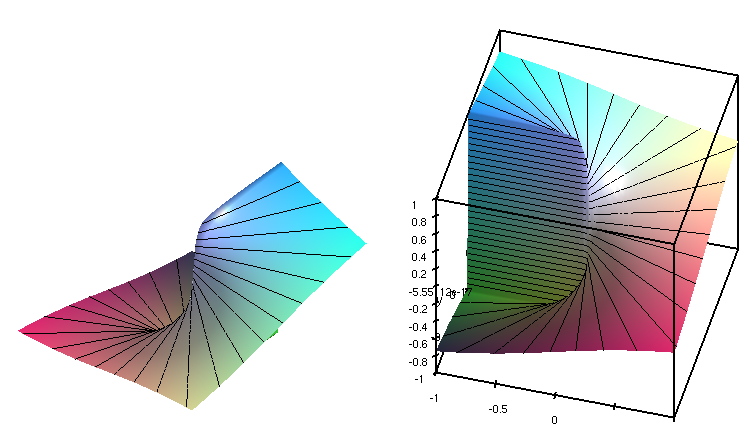
#Whitney Umbrella:
plot3d([u*v, u, v^2],
u=-1..1,
v=-1..1,
title=`The Whitney Umbrella`);
#cross cap:
x := sin(u) * sin(2*v) / 2;
y := sin(2*u) * cos(v)^2;
z := cos(2*u) * cos(v)^2;
# the complete surface:
plot([x,y,z],
u=0..Pi,
v=-Pi/2..Pi/2,
title=`The cross cap`);
# the sectioned surface:
plot([x,y,z],
u=0..Pi,
v=-Pi/2..Pi/2,
view=-1..0.5,
title=`The cross cap split open`);
restart; # cleanup:
#Dini's surface of constant negative curvature :
x := cos(u) * sin(v);
y := sin(u) * sin(v);
z := cos(v) + log(tan(v/2)) + 0.2 * u;
plot([x,y,z], u=0..4*Pi, v=0.1..Pi/2,
grid=[50,20], title=`Dini's surface`);
restart; # cleanup:
#tangent surface of a helix:
x := cos(t); y := sin(t); z := t;
xp := -sin(t); yp := cos(t); zp := 1;
plot3d([x + v*xp, y + v*yp, z + v*zp],
t=0..2*Pi, v=-4..4);
restart; # cleanup:
#Bour's Minimal Surface:
x := r*cos(t)-r^2*cos(2*t)/2;
y := -r*sin(t)-r^2*sin(2*t)/2;
z := (4/3)*r^(3/2)*cos(3*t/2);
plot([x,y,z], t=0..4*Pi, r=1..4,grid=[100,10],style=patch);
restart; # cleanup:
#the Klein bottle :
top := plot3d([(2.5 + 1.5*cos(v))*cos(u),
(2.5 + 1.5*cos(v))*sin(u), -2.5 *sin(v)],
u = 0.. 2* Pi,
v = Pi .. 2*Pi);
middle := plot3d([ (2.5 + 1.5*cos(v)) * cos(u),
(2.5 + 1.5*cos(v)) * sin(u), 3*v- 6 * Pi ],
u = 0.. 2* Pi,
v = Pi .. 2*Pi);
handle := plot3d( [ 2 - 2*cos(v) + sin(u), cos(u),
3 * v - 6 * Pi],
u = 0..2*Pi ,
v = Pi .. 2*Pi);
bottom := plot3d( [2 + (2 + cos(u))*cos(v),sin(u),
-3 * Pi + (2 + cos(u)) * sin(v) ],
u = 0.. 2* Pi,
v = Pi .. 2*Pi);
display([bottom, middle, handle, top]);
restart; # cleanup:
#pumpkin:
plot3d(1+(1/3)*sin(2*theta)*sin(5*phi)^2,
phi=0..2*Pi,
theta=0..Pi,
coords=spherical,
grid=[60,60]);
#helix:
plot3d(3+sin(5*theta+phi)^2,
phi=0..2*Pi,
theta=0..Pi,
coords=spherical,
grid=[60,60]);
#clover:
plot3d(sin(2*theta+3*phi),
phi=0..2*Pi,
theta=0..Pi,
coords=spherical,
grid=[60,60]);
========================options=========================================
axes= NONE/BOXED/NORMAL/FRAME
axesfont = [HELVETICA,10]
color = "red"/"MidnightBlue"/"#009000"
contours = 10
coords = CARTESIAN/SPHERICAL/CYLINDRICAL/Z_CYLINDRICAL.
font = [HELVETICA,10] ROMAN, BOLD, ITALIC or BOLDITALIC.
For HELVETICA and COURIER style may be omitted
orBOLD/OBLIQUE/BOLDOBLIQUE
grid = [25,25]
gridstyle = RECTANGULAR/TRIANGULAR/X_GRIDLINES/Y_GRIDLINES.
labelfont = [HELVETICA,12]
labels = [x,y,z] x, y, and z must be strings. The default
linewidth = n
numpoints = 60.
orientation = [45,45]
pointsize = 3
scaling = UNCONSTRAINED/CONSTRAINED
shading = XYZ, XY, Z, ZGREYSCALE, ZHUE, NONE.
style = POINT/HIDDEN/PATCH/WIREFRAME/CONTOUR/PATCHNOGRID/PATCHCONTOUR/LINE.
thickness = 1
tickmarks = [5,5,5]
title = a title string. \n acts as a line break within string
titlefont = [HELVETICA,BOLDOBLIQUE,14]
tuberadius = 1.0
tubepoints = 16
view = zmin..zmax or view=[xmin..xmax,ymin..ymax,zmin..zmax]
========================================================================
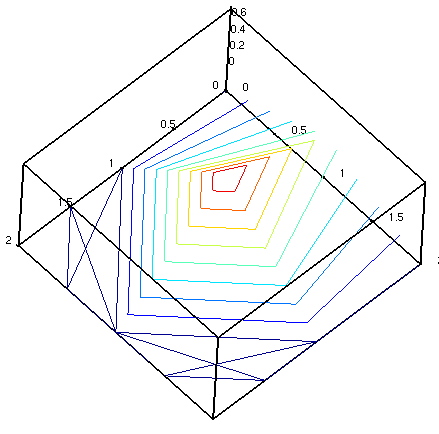
#Plot A File :
dataplot(g432, shading=zgrayscale , gridstyle = TRIANGULAR, style = PATCH);
dataplot(g432, shading = Z , gridstyle = TRIANGULAR, style = HIDDEN);
dataplot(g432, shading = Z , gridstyle = RECTANGULAR, style = PATCHNOGRID);
dataplot(g432, shading = Z , gridstyle = TRIANGULAR, style = PATCHCONTOUR);
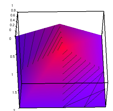
dataplot(g432, shading = Z
, gridstyle = Y_GRIDLINES, style = PATCH);
dataplot(g432, shading = Z , gridstyle = X_GRIDLINES, style = PATCH);
dataplot(g432, shading = Z , gridstyle = Y_GRIDLINES, style = CONTOUR);
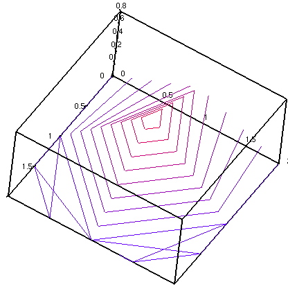
dataplot(g432, shading = Z , gridstyle = Y_GRIDLINES, style = PATCHNOGRID);
dataplot(g432, shading = ZHUE , gridstyle = X_GRIDLINES, style = CONTOUR);
> dataplot(g432, shading = XYZ , gridstyle = RECTANGULAR, style = PATCH);
dataplot(g432, shading = Z , gridstyle = TRIANGULAR, style = WIREFRAME);
dataplot(g431);
TITLE "An optional title"
SURF m n
x11 y11 z11 x12 y12 z12 ... x1n y1n z1n
x21 y21 z21 x22 y22 z22 ... x2n y2n z2n
...
xm1 ym1 zm1 xm2 ym2 zm2 ... xmn ymn zmn
x y z x y z x y z
SURF 3 3
0 0 0 0 1 0 0 2 0
1 0 0 1 1 1 1 2 0
2 0 0 2 1 0 2 2 0